import pandas as pd
import numpy as np
import matplotlib.pyplot as plt
import seaborn as sns
from scipy import stats
from sklearn.preprocessing import LabelEncoder

from warnings import filterwarnings
filterwarnings(action="ignore", category=FutureWarning)

# Load the dataset in a pandas dataframe
dataset = pd.read_csv("book_assets/dataset/data.csv")

class EDA:
    def __init__(self, df) -> None:
        self.df = df
        # Split the dataset into features and targets
        self.features = df.iloc[:, 0:9]
        self.targets  = df.iloc[:, 9:]

        # Split the features into numerical predictors and categorical predictors
        self.categorical_predictors = self.features.select_dtypes(include="object")
        self.numerical_predictors   = self.features.select_dtypes(include="number")

    def check_missing_counts(self):
        return pd.DataFrame(self.df.isna().sum(), columns=["Missing Counts"])


    def check_duplicated_rows(self) -> int:
        return self.df.duplicated().sum()


    def check_outliers(self, n_sigma_limit=3):
        cl = self.df.mean()
        ll = cl - n_sigma_limit * self.df.std()
        ul = cl + n_sigma_limit * self.df.std()

        below_ll = (self.df < ll).sum()
        above_ul = (self.df > ul).sum()

        return pd.concat(
            objs = [cl, ll, ul, below_ll, above_ul],
            axis = 1,
            keys = [
                "Mean",
                "Lower Limit(LL)",
                "Upper Limit (UL)",
                "Below LL",
                "Above UL"]
        ).dropna()


    def check_normality(self):
        alpha = 0.05
        normality_test_df = pd.DataFrame(
            columns=[
                "Feature",
                "Statistic",
                "p-value",
                "Null Hypothesis"
            ]
        )

        for predictor in self.numerical_predictors.columns:
            stat, pval = stats.normaltest(self.numerical_predictors[predictor])

            normality_test_df.loc[len(normality_test_df)] = [
                predictor,
                stat,
                pval,
                "Reject" if pval <= alpha else "Accept"
            ]

        return normality_test_df


    def check_categorical_class_names(self):
        for predictor in self.categorical_predictors:
            print(predictor, self.categorical_predictors[predictor].unique())


    def check_categorical_class_balance(self):
        df = pd.DataFrame(columns=[
            "Predictor",
            "Class",
            "Frequency",
            "Total Observations",
            "Class Proportion"
        ])
        for predictor_name in self.categorical_predictors.columns:
            predictor = self.categorical_predictors[predictor_name]
            predictor_classes = predictor.unique()
            predictor_nclasses = len(predictor_classes)

            for predictor_class in predictor_classes:
                class_freq = len(predictor[predictor == predictor_class])
                total_items = len(predictor)
                class_prop = class_freq / total_items

                df.loc[len(df)] = [
                    predictor_name,
                    predictor_class,
                    class_freq,
                    total_items,
                    class_prop
                ]

        return df


    def check_categorical_class_distribution(self):
        return self.df.groupby(["material", "infill_pattern"]).count().T

    def interpret_corr(self, corr):
        corr_interpretation = ""

        # Interpret the correlation
        if np.abs(corr) == 0:
            corr_interpretation = "No Correlation"
        elif np.abs(corr) > 0 and np.abs(corr) < 0.2:
            corr_interpretation = "Very Weak Correlation"
        elif np.abs(corr) >= 0.2 and np.abs(corr) < 0.4:
            corr_interpretation = "Weak Correlation"
        elif np.abs(corr) >= 0.4 and np.abs(corr) < 0.6:
            corr_interpretation = "Moderately Strong Correlation"
        elif np.abs(corr) >= 0.6 and np.abs(corr) < 0.8:
            corr_interpretation = "Strong Correlation"
        elif np.abs(corr) >= 0.8 and np.abs(corr) < 1.0:
            corr_interpretation = "Very Strong Correlation"
        elif np.abs(corr) == 1.0:
            corr_interpretation = "Perfect Correlation"

        return corr_interpretation

    def check_corr_of_features_and_targets(self, only_strong=False):
        df = pd.DataFrame(columns=["Target", "Feature", "Pearson (r)", "Remarks"])
        for target in self.targets.columns:
            for feature in self.features.columns:
                if feature in self.numerical_predictors.columns:
                    # Calculate the correlation
                    corr = self.targets[target].corr(self.features[feature])

                    # Append the result
                    df.loc[len(df)] = [
                        target,
                        feature,
                        corr,
                        self.interpret_corr(corr)
                    ]

        # Return the final dataframe
        if only_strong:
            return df[(
                    df["Pearson (r)"].abs() >= 0.4
                )].sort_values(by=["Target", "Pearson (r)"])
        else:
            return df.sort_values(by=["Target", "Pearson (r)"])

    def check_assoc_of_features_and_targets(self):
        label_encoder = LabelEncoder()
        df = pd.DataFrame(columns=["Target", "Feature", "Point Biserial (r)", "Remarks"])
        for target in self.targets.columns:
            for feature in self.features.columns:
                if feature in self.categorical_predictors.columns:
                    x = self.features[feature]
                    y =  self.targets[target]

                    label_encoder.fit(x)

                    stat, pval = stats.pointbiserialr(label_encoder.transform(x), y)

                    df.loc[len(df)] = [
                        target,
                        feature,
                        stat,
                        self.interpret_corr(stat)
                    ]

        return df.sort_values(by=["Target", "Point Biserial (r)"])

    def check_feature_multicorr(self):
        corr = self.numerical_predictors.corr()
        sns.heatmap(corr, annot=True)


    def visualize_numerical_predictors(self):
        # | fig-cap: Histogram of the Numerical Features. Based on above data, majority of our features were not normally distributed. This is in-fact natural since most of the features were machine parameters settings.
        for i in range(len(self.numerical_predictors.columns)):
            for j in range(len(self.numerical_predictors.columns)):
                feature_index = i+j+1
                if feature_index < len(self.numerical_predictors.columns):
                    plt.subplot(3,2,feature_index)
                    sns.kdeplot(self.numerical_predictors.iloc[:,feature_index])
                    sns.histplot(self.numerical_predictors.iloc[:,feature_index], stat="density")
                    plt.tight_layout()
                else:
                    break

    def visualize_targets(self):
        fig, ax = plt.subplots(3,1)
        fig.tight_layout()
        for i in range(len(self.targets.columns)):
            sns.kdeplot(self.targets.iloc[:, i], ax=ax[i])
            sns.histplot(self.targets.iloc[:, i], ax=ax[i], stat="density")


    def visualize_outliers(self):
        sns.boxplot(data=self.df)
        plt.xticks(rotation=90)

    def visualize_class_distribution(self):
        sns.histplot(self.df, x="material", hue="infill_pattern", multiple='dodge')

    def visualize_targets_dist(self, by):
        for i in range(len(self.targets.columns)):
            plt.subplot(1,3,i+1)
            plt.tight_layout()
            sns.boxplot(data=self.df, x=by, y=self.targets.columns[i])

eda = EDA(df=dataset)1 Exploratory Data Analysis
1.1 Introduction
Welcome to the exciting EDA phase of our project! In this section, we’ll dive deep into the 3D Printer Dataset for Mechanical Engineers and uncover fascinating insights. First, we’ll familiarize ourselves with the dataset’s feature and target variables to get a better understanding of the data we’re working with. Then, we’ll explore the data further to identify any potential machine learning modeling issues that we might encounter as we proceed to the regression phase of this project. Are you ready to join us on this journey of discovery? Let’s get started!
1.2 About the Dataset
The 3D Printer Dataset for Mechanical Engineers(Okudan (2016)) is dataset for those who want to find relations between the input parameters of 3D printers and the output quality, accuracy and strength of the printed objects¹. It was generated by Ahmet Okudan, a senior engineer at Numesys and a mechanical engineering researcher at Selcuk University in Turkey.
The dataset has nine feature variables and three target variables.
1.2.1 Features
- Layer Height (mm): The thickness of each layer of the printed object
- Wall Thickness (mm): The thickness of the outer shell of the printed object
- Infill Density (%): The percentage of the interior volume of the printed object that is filled with material
- Infill Pattern: The shape of the infill material, such as grid, honeycomb, triangles, etc.
- Nozzle Temperature (Cº): The temperature of the extruder nozzle that melts and deposits the material
- Bed Temperature (Cº): The temperature of the platform that supports the printed object
- Print Speed (mm/s): The speed at which the nozzle moves along the X-Y plane
- Material: The type of filament material used for printing, such as PLA, ABS, PETG, etc.
- Fan Speed (%): The speed of the cooling fan that reduces the temperature of the printed object
1.2.2 Targets
- Roughness (µm): The average deviation of the surface height from the mean plane
- Tension (ultimate) Strength (MPa): The maximum stress that a material can withstand before breaking
- Elongation (%): The percentage of increase in length that a material undergoes before breaking
1.3 Exploratory Data Analysis
The dataset underwent a thorough exploration and assessment, which included the following steps:
- Verification of missing values to ensure data completeness.
- Identification of duplicated rows to prevent data redundancy.
- Assessment of feature normality to determine the appropriate statistical tests.
- Detection of outliers among the features to prevent skewed results.
- Evaluation of class balance, proportion, and categorical features to ensure data representativeness.
- Investigation of correlations among numerical features to uncover hidden relationships.
- Examination of multi-collinearity among features to prevent model instability.
To facilitate this comprehensive analysis, a central python class named EDA was constructed. For further information about this class, please refer to the code listing below.
1.3.1 Data Summary
Using the EDA class above, the following items were observed from the dataset:
1.3.2 Missing and Duplicate Values:
The dataset was found to have no missing values and duplicated rows.
eda.check_missing_counts()| Missing Counts | |
|---|---|
| layer_height | 0 |
| wall_thickness | 0 |
| infill_density | 0 |
| infill_pattern | 0 |
| nozzle_temperature | 0 |
| bed_temperature | 0 |
| print_speed | 0 |
| material | 0 |
| fan_speed | 0 |
| roughness | 0 |
| tension_strenght | 0 |
| elongation | 0 |
print(f"Number of duplicated rows: {eda.check_duplicated_rows()}-rows")Number of duplicated rows: 0-rows1.3.3 Normality Check
In terms of its empirical distribution, the dataset was tested for normality using the D’Agostino and Pearson’s test implemented in scipy.stats.normaltest. Based on the result of the test, the three target variables nozzle_temperature, roughness, and elongation have sufficient evidence at 5% significance level that they were drawn from a normal distribution. All of the numerical predictors were not normally distributed. This is expected since all of the predictors were machine parameter settings.
eda.visualize_targets()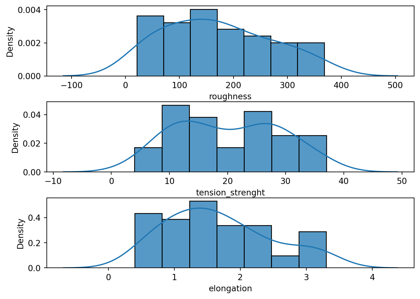
tension_strength variable.eda.visualize_numerical_predictors()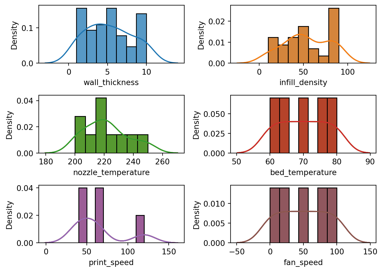
eda.check_normality()| Feature | Statistic | p-value | Null Hypothesis | |
|---|---|---|---|---|
| 0 | layer_height | 17.231029 | 0.000181 | Reject |
| 1 | wall_thickness | 8.034294 | 0.018004 | Reject |
| 2 | infill_density | 6.650689 | 0.035960 | Reject |
| 3 | nozzle_temperature | 2.890296 | 0.235711 | Accept |
| 4 | bed_temperature | 18.617248 | 0.000091 | Reject |
| 5 | print_speed | 10.203504 | 0.006086 | Reject |
| 6 | fan_speed | 18.617248 | 0.000091 | Reject |
Tabulated results of the D’Agostino and Pearson’s test. Based on the results, at 5% significance, we have enough statistical evidence that all of our feature variables were not drawn from a normal distribution. On the other hand, at the same level of statistical significance, we don’t have enough statistical evidence to reject the null hypthesis that our target variables were drawn from a normal distribution.
1.3.4 Outliers
In this dataset, outliers were defined as a univariate datapoint that exists outside the 3 sigma limits (\(\bar{x}\pm3\sigma\)) from the mean. Based on the result of EDA, the dataset does not contain outliers outside the defined limits.
eda.visualize_outliers()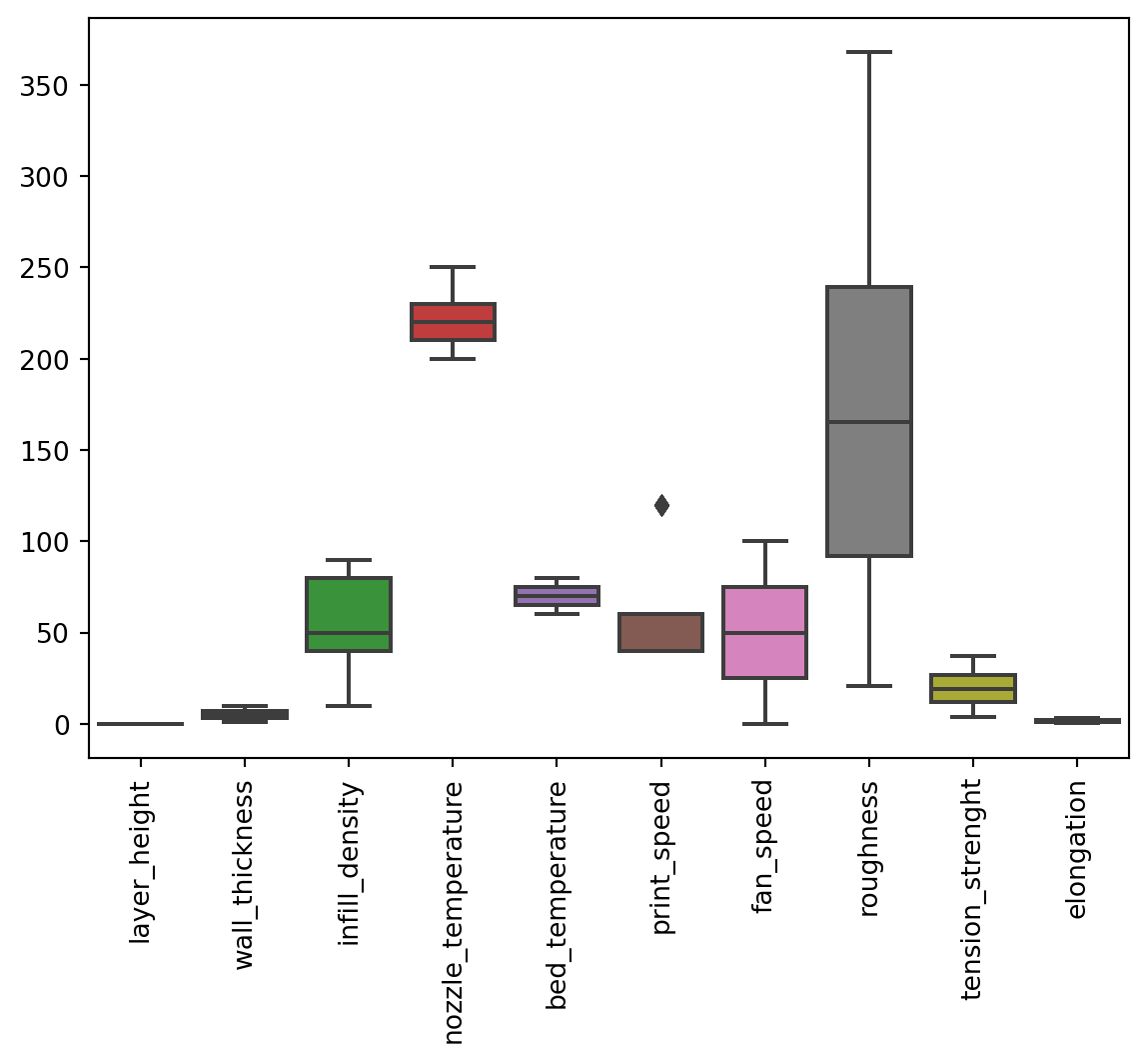
print_speed seems to have an outlier however, this value does not fall outside the \(3\sigma\) limits.eda.check_outliers()| Mean | Lower Limit(LL) | Upper Limit (UL) | Below LL | Above UL | |
|---|---|---|---|---|---|
| layer_height | 0.106 | -0.087190 | 0.299190 | 0 | 0 |
| wall_thickness | 5.220 | -3.548240 | 13.988240 | 0 | 0 |
| infill_density | 53.400 | -22.690440 | 129.490440 | 0 | 0 |
| nozzle_temperature | 221.500 | 177.038942 | 265.961058 | 0 | 0 |
| bed_temperature | 70.000 | 48.571429 | 91.428571 | 0 | 0 |
| print_speed | 64.000 | -25.076899 | 153.076899 | 0 | 0 |
| fan_speed | 50.000 | -57.142857 | 157.142857 | 0 | 0 |
| roughness | 170.580 | -126.522388 | 467.682388 | 0 | 0 |
| tension_strenght | 20.080 | -6.696901 | 46.856901 | 0 | 0 |
| elongation | 1.672 | -0.692565 | 4.036565 | 0 | 0 |
Tabulated result of outlier checking. Based on the above results, there was not outliers that fall outside the \(3\sigma\) limits
1.3.5 Balance of Categorical Classes
Upon inspection of class distribution, it was found that for both material, and infill_pattern, the proportion of their respective classes were balanced at 50% proportion each.
eda.check_categorical_class_balance()| Predictor | Class | Frequency | Total Observations | Class Proportion | |
|---|---|---|---|---|---|
| 0 | infill_pattern | grid | 25 | 50 | 0.5 |
| 1 | infill_pattern | honeycomb | 25 | 50 | 0.5 |
| 2 | material | abs | 25 | 50 | 0.5 |
| 3 | material | pla | 25 | 50 | 0.5 |
Result of counting class frequencies per categorical features. Based on above results, each of the classess has a 50-50 proportion.
eda.visualize_class_distribution()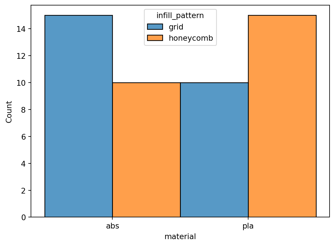
eda.check_categorical_class_distribution()| material | abs | pla | ||
|---|---|---|---|---|
| infill_pattern | grid | honeycomb | grid | honeycomb |
| layer_height | 15 | 10 | 10 | 15 |
| wall_thickness | 15 | 10 | 10 | 15 |
| infill_density | 15 | 10 | 10 | 15 |
| nozzle_temperature | 15 | 10 | 10 | 15 |
| bed_temperature | 15 | 10 | 10 | 15 |
| print_speed | 15 | 10 | 10 | 15 |
| fan_speed | 15 | 10 | 10 | 15 |
| roughness | 15 | 10 | 10 | 15 |
| tension_strenght | 15 | 10 | 10 | 15 |
| elongation | 15 | 10 | 10 | 15 |
Tabulation of class heirarchical distribution supporting the histogram above.
1.3.6 Correlation of Numeric Features with Targets
In terms of correlation among features and targets, it was found that nozzle_temperatureand layer_height had a moderately strong correlation with printing elongation. As the nozzle_temperature increased, printing elongation tended to decrease. In contrast, as the layer_height increased, printing elongation also tended to increase. Furthermore, as the layer_height increased, so did the printing roughness. Lastly, as the nozzle_temperature decreased, the printing tensile_strength tended to increase.
eda.check_corr_of_features_and_targets()| Target | Feature | Pearson (r) | Remarks | |
|---|---|---|---|---|
| 17 | elongation | nozzle_temperature | -0.527447 | Moderately Strong Correlation |
| 18 | elongation | bed_temperature | -0.300871 | Weak Correlation |
| 20 | elongation | fan_speed | -0.300871 | Weak Correlation |
| 19 | elongation | print_speed | -0.234052 | Weak Correlation |
| 16 | elongation | infill_density | 0.159009 | Very Weak Correlation |
| 15 | elongation | wall_thickness | 0.176364 | Very Weak Correlation |
| 14 | elongation | layer_height | 0.507583 | Moderately Strong Correlation |
| 1 | roughness | wall_thickness | -0.226987 | Weak Correlation |
| 2 | roughness | infill_density | 0.118389 | Very Weak Correlation |
| 5 | roughness | print_speed | 0.121066 | Very Weak Correlation |
| 4 | roughness | bed_temperature | 0.192142 | Very Weak Correlation |
| 6 | roughness | fan_speed | 0.192142 | Very Weak Correlation |
| 3 | roughness | nozzle_temperature | 0.348611 | Weak Correlation |
| 0 | roughness | layer_height | 0.801341 | Very Strong Correlation |
| 10 | tension_strenght | nozzle_temperature | -0.405908 | Moderately Strong Correlation |
| 12 | tension_strenght | print_speed | -0.264590 | Weak Correlation |
| 11 | tension_strenght | bed_temperature | -0.252883 | Weak Correlation |
| 13 | tension_strenght | fan_speed | -0.252883 | Weak Correlation |
| 7 | tension_strenght | layer_height | 0.338230 | Weak Correlation |
| 9 | tension_strenght | infill_density | 0.358464 | Weak Correlation |
| 8 | tension_strenght | wall_thickness | 0.399849 | Weak Correlation |
Correlation table between features and targets
eda.check_corr_of_features_and_targets(only_strong=True)| Target | Feature | Pearson (r) | Remarks | |
|---|---|---|---|---|
| 17 | elongation | nozzle_temperature | -0.527447 | Moderately Strong Correlation |
| 14 | elongation | layer_height | 0.507583 | Moderately Strong Correlation |
| 0 | roughness | layer_height | 0.801341 | Very Strong Correlation |
| 10 | tension_strenght | nozzle_temperature | -0.405908 | Moderately Strong Correlation |
Correlation table between features and targets showing only those with strong correlations and above.
1.3.7 Association of Categorical Features with Targets
Upon checking the association of categorical features with the target variables, it was found that neither material nor infill_pattern had a moderately strong association with any of the target variables. However, looking at the point biserial correlation coefficient, elongation, roughness, and tensile_strength had a weak correlation with the material used.
eda.check_assoc_of_features_and_targets()| Target | Feature | Point Biserial (r) | Remarks | |
|---|---|---|---|---|
| 4 | elongation | infill_pattern | 0.046138 | Very Weak Correlation |
| 5 | elongation | material | 0.394737 | Weak Correlation |
| 1 | roughness | material | -0.233173 | Weak Correlation |
| 0 | roughness | infill_pattern | -0.068340 | Very Weak Correlation |
| 2 | tension_strenght | infill_pattern | 0.009054 | Very Weak Correlation |
| 3 | tension_strenght | material | 0.289726 | Weak Correlation |
Association table between features and targets
1.3.8 Multicollinearity Among Numerical Features
Upon checking of collinearity among the features, it was found that bed_temparature and fan_speed were perfectly correlated. Furthermore, nozzle_temparature was strongly correlated with bed_temparature and fan_speed since both were perfectly correlated.
eda.check_feature_multicorr()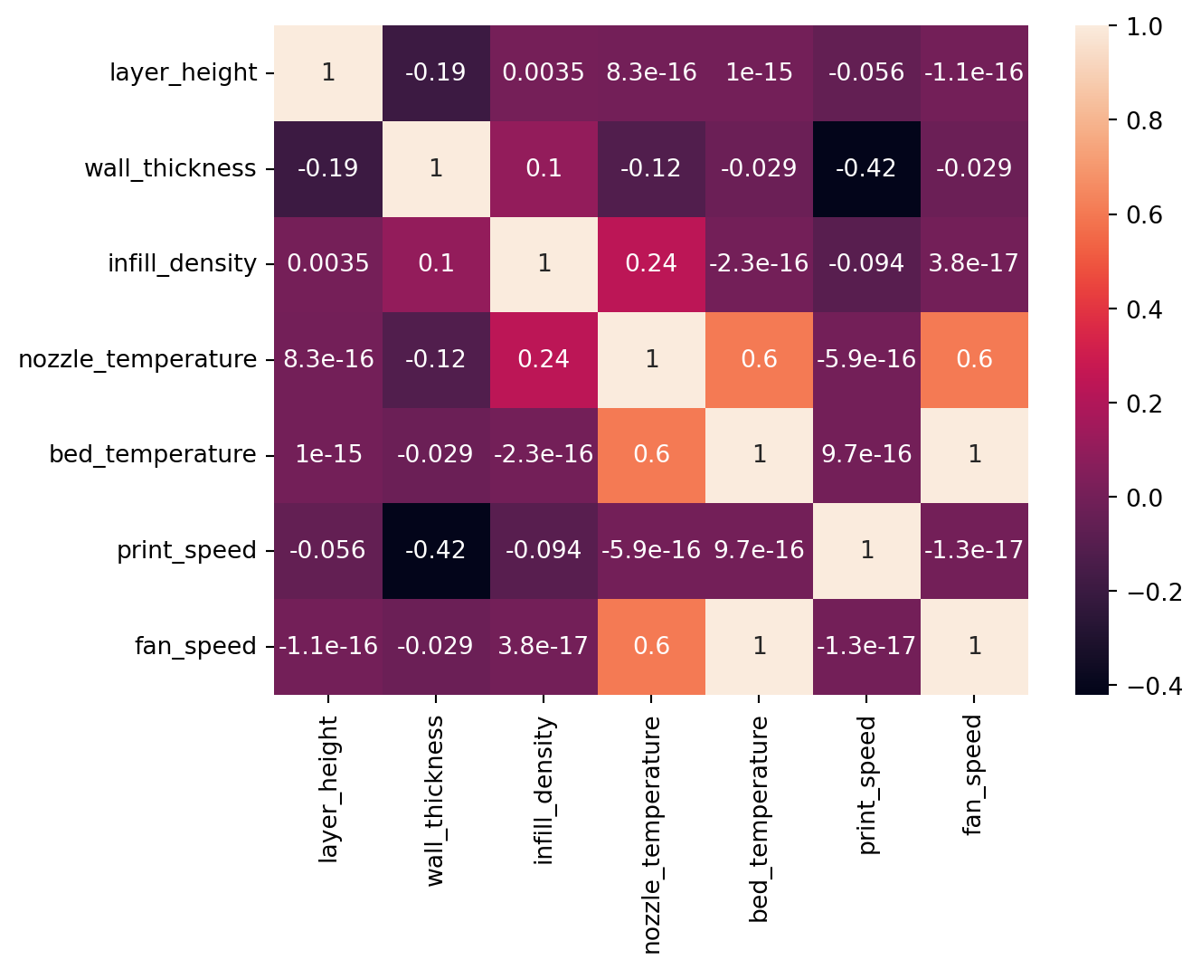
1.4 Conclusion
In this section, we explored the 3D Printer dataset using both univariate and bivariate EDA methods. Our exploration revealed that the dataset is relatively small, simple, and clean, requiring minimal data preprocessing aside from feature scaling and categorical encoding. In the next section, we will preprocess this dataset and use it in a series of linear models to quantify the impact of each machine setting on printing quality. Stay tuned for our exciting findings!